First Steps with PyTorch
Through the use of Machine Learning, and particularly Deep Learning, the range of activities that computers are capable of performing has exploded. Examples include the ability for computer vision systems to analyze an image and describe in plain English what it contains, for AI agents to play complex strategy games, or to accurately diagnose medical scans with accuracy that rivals trained physicians.
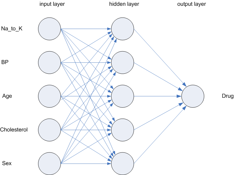
Deep Learning makes use of artificial neural networks, which are computer simulations patterned after the human brain. Such networks consist of thousands, or even millions of nodes that communicate and interact with one another. The nodes are organized through layers that allow for the simulation to interpret the data moving through the network. Nodes in each layer are connected to nodes in other layers through association. The associations are called weights and their linkage controls the decision that the network will make about the data.
Such networks can be efficiently modeled using multi-dimensional arrays, such as those provided by the NumPy, TensorFlow, and PyTorch libraries in Python. Such libraries usually provide a core data structure, such as the Tensor in PyTorch, and a set of features that allow for the efficient design and training of a network. Libraries directly aimed at Deep Learning, such as TensorFlow and PyTorch, also provide packages to tackle some of the challenges of creating complex models such as cluster based/distributed training, efficient data loading, hardware acceleration of mathematical functions, and utilities to help with common deep learning functions.
In this blog post, we'll look at how you can get up and running with one of the most popular Deep Learning libraries: PyTorch. We'll describe the core components, look at how PyTorch can be used to load an already trained model, create a simple image pipeline that will prepare data for analysis, and apply the model to the data.
Background: What is Deep Learning?
This article is primarily focused on how to use Deep Learning tools. Before wading out of the shallows, though, it is very helpful to understand what Deep Learning is. In traditional (or classical) machine learning, we are interested in utilizing statistical techniques to understand how input "features" contribute to the underlying statistical variance of an outcome (called a target), and using that relationship to come up with correct outcomes on new data.
When building a classical machine learning model, while some work might go choosing which machine learning algorithm to use and the best choice of algorithmic parameters, the most important decisions involve which set of features to include as inputs. These sets of choices are sometimes called "feature engineering." Tremendous amounts of time will be spent inspecting features, combining datasets, assessing correlation, encoding, and cleaning.
Deep learning, in contrast, works very differently. Instead of hand-tuning the features and trying to decide which are most important to the target, those decisions are delegated to the computer. Neural nets are able to ingest raw data and find useful representations which contribute to the outcome of interest. At lower levels in the network, these inferences may be abstract. As you move toward higher levels in the network, though, they often begin to take meaningful patterns in the form of edges or features (such as eyes, ears, or object attributes). In fact, attempting to inject additional features may not even be desirable as the machine is often very good at drawing its own inferences.
This ability for the model to draw its own inferences is transformational. Its this ability that makes Deep Learning so powerful, and also a little bit mysterious.
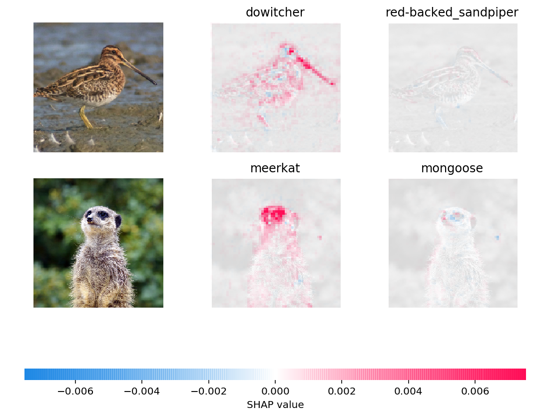
Aidse: Historically, understanding why Deep Learning models draw the conclusions they do has been difficult, though this is starting to change. Using libraries such as Shap, it's possible to inspect how the model perceives the input data and what features may have contributed to a specific outcome. The figure below shows the predictions for two input images are explained by the presence of certain attributes. Red pixels represent positive contributions to the label probability while blue pixels represent negative contributions. In the case of the bird image, the model recognizes the presence of a narrow beak and certain patterns in the plumage, patterns which are not seen in the next most likely label (red-backed_sandpiper). In the case of the meerkat image, it recognizes the wide striping around the eyes.
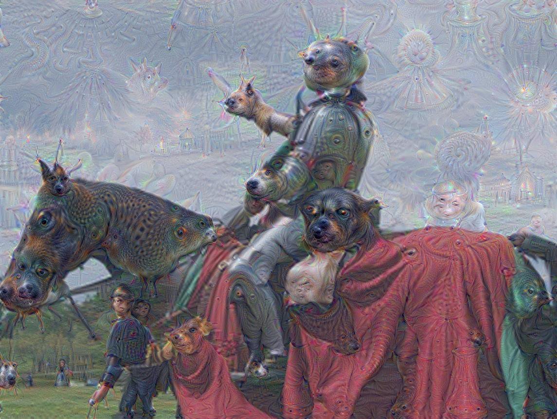
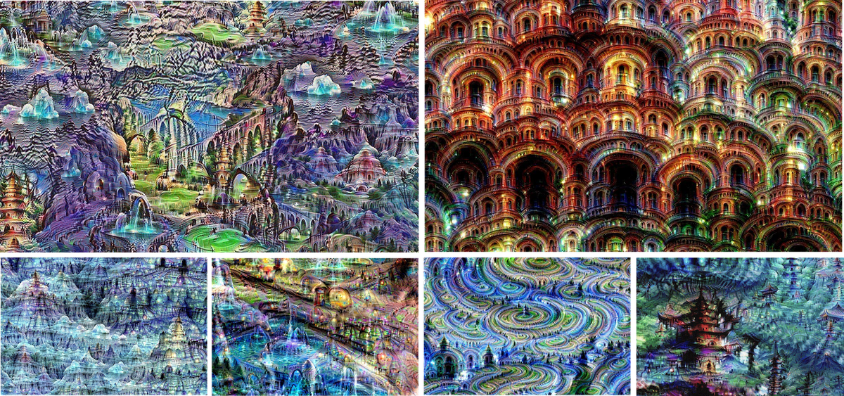
It's worth noting that it's not always possible to directly inspect why the machine came to the conclusions it did. The second set of images show a network that has been run in reverse, where it was asked to draw a picture based on a particular label of interest. The top example shows what came out when asked about a "knight" while the second shows how the AI perceives "buildings."
How Deep Learning Networks Work
At their heart, Deep Learning networks provide a way to take data in some form and produce data in another form such as labels, numbers, text, or additional images. The output of one network can then be used as the input for a new layer that allows for additional transformation.This is where the "deep" part of the network comes from. A Deep Network has "hidden layers," that become difficult to inspect. Going one step further, the output of a deep model can be piped into the input of a classical machine learning technique as a set of input features.
As data moves through the network, it is modeled as a set of floating point numbers that characterize the structure of the data. Nearly any type of data can be modeled including images, video (as a set of images), sound, and raw text. As the data moves through the network, it is combined with the weights of previous layers of neurons and will (eventually) map to an output target of interest. A "solution" to the network is found by trying weights until a map is found that produces a desired output structure.
The following videos from 3Blue1Brown explain the internal structures of neural networks more in depth and provide the mathematical details of how a network converges during training.
Consuming a Deep Learning Model
Often the first step in working with a Deep Learning tool is to consume an existing model created by someone else. It's much the same as the creation of a "Hello World" program is the first step for aspiring developers. Consuming someone else's model allows you to understand the mechanics of loading the model's structure to a form which can be executed, preparing data for processing, and managing the control structures needed for a machine learning program.
In the remainder of this article, we will look at what is involved to apply a state of the art neural network trained for image recognition to a new set of images. We will show how to load the model from the set of pre-trained models interface included with torchvision, create a simple image processing pipeline that will standardize inputs into the format expected by the model, load image data and convert it into a tensor representation, apply the model, and retrieve the results and confidences.
ImageNet
The network we will be working with was trained on the ImageNet database as part of an image classification contest called the Large Scale Visual Recognition Challenge (ILSVRC). ImageNet includes about fourteen million images tagged with information about the objects they contain.
PyTorch includes a number of models that were trained on the ImageNet datset, all of which can be loaded using the models package. We will be using the ResNet101 network, which utilizes some 44.5 million parameters in its network. ResNet101 was released in November 2014 and was one of the top-performing models for ImageNet in 2015.
Dependencies and Supporting Tools
While the soul of an ML program is the model, nearly all ML programs require supporting structure to work correctly. These include routines to retrieve and transform data, handle the input/output interfaces, and initialize processing pipelines.
Python includes a wealth of utilities that can provide this functionality through an easy to consume API. The dependencies that we will use in this example include:
torch: the PyTorce library which provides model implementations and theTensorconstructtorchvisionandtorchvision.models: the PyTorch computer vision librarytorchvision.transforms: a library of image processing utilities that can be used to prepare data for consumption from PyTorchPIL: the Python Imaging Library, a popular library for working with Images in Pythonrequests: a Python HTTP client, which can be used to retrieve data from the webio.BytesIO: one of Python's core tools for working with streams, which implements a file-like object for binary data objects that can be used to interact with PyTorch interfaces that expect a file handle
# PyTorch components
import torch
from torchvision import models

# matplotlib utilities for visualizing the results
import matplotlib.pyplot as plt

# PyTorch Transform Functions
from torchvision import transforms

# PyTorch uses PIL to work with images
from PIL import Image

# requests is an http library used for fetching remote data
import requests

# BytesIO is an in-memory string implementation that can be used
# to provide a file-like object for binary data
from io import BytesIO
Retrieving Pre-Trained Models
torchvision.models contains definitions of models for addressing different types of image processing tasks. These include: image classification, pixelwise semantic segmentation, object detection, instance segmentation, person keypoint detection, and video classification. You can initialize instances of specific types of models by calling a helper method like models.alexnet or models.densenet161.
We will be using a variant of models.resnet101, which will initialize a 101 layer convolutional neural network (CNN) trained on more than a million images from the ImageNet dataset.
# Import ResNet from pre-trained models
resnet = models.resnet101(pretrained=True)
If you have not used the model instance previously, it must first download a copy of the weights before it can initialize. This is a one-time operation, the weights will be cached locally for use in the future.
Creating a Processing Pipeline
To obtain the best results from the model, we need to do a degree of processing. The model needs the images to be of a uniform size and for the color values to be roughly in the same numerical range in order to return the most accurate results. This is the type of preparatory work that torchvision.transforms was created for. The code in the listing creates a four step pipeline that:
- scales the images to a 256 by 256 pixels
- crops the image to a 224 by 224 pixel square around the center
- transforms the resulting data to a tensor format (a three dimensional array with red, green, and blue components each encoded in a separate channel)
- normalizes the channel value distribution to a known average and standard deviation
# Create image processing pipeline so that all input images have same paremeters
# Step 1: Resize and Center (Resize: 256x256, Crop: 224x224 around the center)
# Step 2: Convert to Tensor Input Format
# Step 3: Normalize Color Inputs
preprocess = transforms.Compose([
    transforms.Resize(256),
    transforms.CenterCrop(224),
    transforms.ToTensor(),
    transforms.Normalize(
        mean=[0.485, 0.456, 0.406],
        std=[0.229, 0.224, 0.2525])
])
Retrieve Data for Processing
PyTorch is able to consume data from any standard Python file-like object. File-like objects are the standard input/output interface used by Python. They implement methods like read, write, and seek. The data might be stored on a local file system, or be part of an object storage or website. The code in the example shows how to use requests to retrieve an image from a website, initialize a stream from the results, and create an PIL.Image instance which will decode the data into a format that can be consumed by PyTorch.
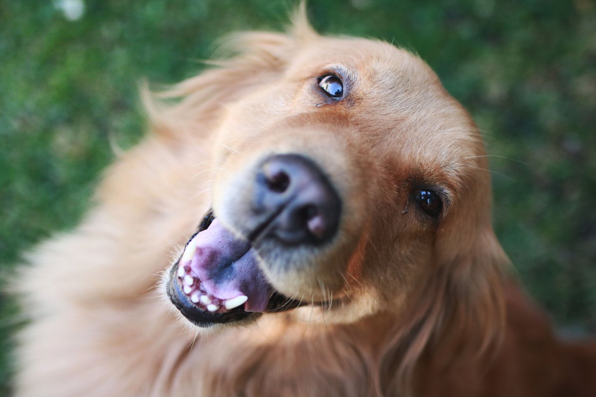
# Retrieve picture of Golden Retriever from website, create PIL image representation
# of the data using BytesIO as an intermediary file-like object
r = requests.get('https://oak-tree.tech/documents/116/resnet.golden-retriever.jpg')
rimg = Image.open(BytesIO(r.content))
Classify Image With ResNet101
With the pre-processing pipeline prepared and the image data retrieved for use locally, we can apply the model. The code in the listing:
- invokes the
preprocessingmethod which scales, crops, converts, and normalizes - calls
unsqueezeon the tensor output from the pipeline, which inserts a new dimension that will encode the batch - configures the trained model to run on new-data (putting it in "inference" mode) by calling
eval - classifies the model
# Pass image through pre-processing pipeline before using model
rimg_t = preprocess(rimg)
rbatch_t = torch.unsqueeze(rimg_t, 0)

# Configure model to work on new-data (inference) by putting model in eval mode
_ = resnet.eval()

# Classify the image using model
out = resnet(rbatch_t)
Interpreting the Results
Calling the resnet method on the batch input image executed a set of tens of millions of operations and returned a set of 1000 scores, each one corresponding to the 1000 labels on which the data was trained. How do you go about interpreting the results and determining what the model saw in the image?
To compare what the model predicted for the labels, we can retrieve an ordered text file which uses the same order as the model. Then, we can find the highest ranking labels and pull those from the list.
The code in the listing:
- uses
requestsa second time to retrieve the list of labels and unpack it to a Python list - pulls the top result form the model run on the photo and correlates it with the ImageNet labels based on positional index
- merges the label and confidence into a caption that is output to the console
# Retrieve image labels to interpret image output
rlabels = requests.get(
    'https://oak-tree.tech/documents/111/imagenet.target-classes.txt')

# Decode the binary data to a string, split the file into individual labels
# identified by index location, and clean any trailing white space
inetlabels = [s.strip() for s in rlabels.content.decode('utf-8').split('\n')]

# Pull top result from the model run on the photo, correlate with the imagenet labels
# retrieved from online
_, i = torch.max(rout, 1)
pconf = torch.nn.functional.softmax(rout, dim=1)[0]

# Output labels and confidence to the console
print('Object in "dog" photo as identified by ResNet101: %s. Confidence: %s'
    % (inetlabels[i], pconf[i].item()))
Object in "dog" photo as identified by ResNet101: golden retriever. Confidence: 0.8406960368156433
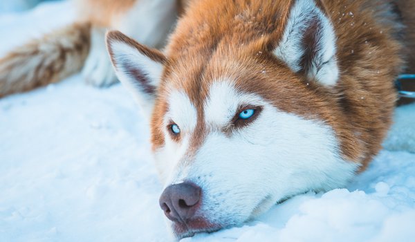
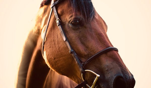
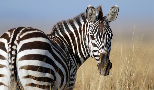
The model correctly identified not just the dog in the photo, but the breed of dog as well. That's pretty impressive! The code below tests it against a larger set of images including a selection of animals pulled from Unsplash.
# Import helper methods for structuring the images and creating
# a figure of the results in Jupyter
from collections import OrderedDict
from matplotlib.pyplot import imshow


# Same model can detect other types of objects other than just dogs.
# The original model was trained on 1000 input labels.
example_images = OrderedDict((
    ('Wolf', 'https://oak-tree.tech/documents/115/resnet.wolf.jpg'),
    ('Horse', 'https://oak-tree.tech/documents/117/resnet.horse-bridle.jpg'),
    ('Zebra', 'https://oak-tree.tech/documents/113/resnet.zebra.jpg'),
    ('Elk', 'https://oak-tree.tech/documents/112/resnet.elk.jpg'),
))


# Set the figure output size
plt.figure(figsize=(30, 30))

# Enumerate and unpack the values in the source data
for i, (a, aurl) in enumerate(example_images.items()):

    # Retrieve data, create image instance, raise an error if the
    # the request failed
    ar = requests.get(aurl)
    if not ar.ok:
        raise ValueError('Unable to retrieve image for %s from %s' % (a, aurl))
    aimg = Image.open(BytesIO(ar.content))

    # Apply image pipeline, create tensor representation
    aimg_t = preprocess(aimg)

    # Unsqueeze image and apply model
    ab_t = torch.unsqueeze(aimg_t, 0)
    aout = resnet(ab_t)

    # Retrieve label and probability of estimate
    _, ai = torch.max(aout, 1)
    aconf = torch.nn.functional.softmax(aout, dim=1)[0]

    # Plot image, human label, and ResNet Label
    plt.subplot(len(example_images)/2+1, 2, i+1)
    plt.title('%s. ResNet Label: %s (%s)' % (a, inetlabels[ai], aconf[ai].item()), fontsize=20)
    imshow(aimg)
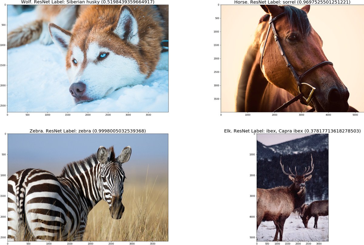
The success of the network depends on how well the subjects were represented in the training set. Of the four images assessed here, the model identified all of the inputs correctly or almost correctly. It selected "siberian husky" for the "wolf" image, which is a very close match. While incorrect, the selection of "capra ibex" isn't so different from "elk," they are both hooved herbivores, after all. That is pretty good accuracy on a set of inputs that the network has never seen before.
Wrapping Up
Knowing how to leverage pre-trained models, in addition to the scaffolding and supporting structure they require, allows you to integrate a neural net without having to design or train it. Neural nets like ResNet101 can provide surprising value to larger systems. This includes examples where they can be used directly, such as in cases where the contents of images might need to be indexed, also in cases which models trained on one dataset can be be used on new data through techniques such as Transfer Learning.
While we've covered a large amount of ground here, Neural Nets and related techniques represent a deep subject. This article article represents the barest tentative steps on the PyTorch path. In future articles, we'll look at the core components of the library and begin to explore ways to train custom models for use in medical image processing and other use-cases.
Comments
Loading
No results found