Modeling Data with NumPy: Image Volumes
In many applications, image data can be combined to create three-dimensional scenes or data volumes. Such data is acquired in a host of different ways: using pictures taken of an object from different perspectives, using special sensors such as LIDAR, or by medical imaging processes like MRI or CT.
Three dimensional data derived from images can be used in many interesting ways, such as:
- more accurate inspection of components at manufacturing sites
- allowing us to see forgotten ruins covered by the jungle
- providing powerful ways for surgeons to more accurately plan and execute complex operations and verify that treatment was successful
- improving the performance and accuracy of robotic surgery
and many more.
Python in general, and NumPy in specific has become important in working with volumetric image data. In this article, we will look at ways in which you can use NumPy to work with a stack of CT images as a cohesive dataset, use features of NumPy such as boolean masks to improve the contrast, and show how to visualize the data as a series.
This article is Part 4 of a larger series showing how NumPy can be used to model data for machine learning and visualization. If you have not already done so, checkout Part 1, which provides an overview of NumPy and how to work with image data. A Jupyter notebook with the code in the article can be downloaded here. A Docker environment with NumPy, Pandas, and other dependencies needed to run the code can be found here.
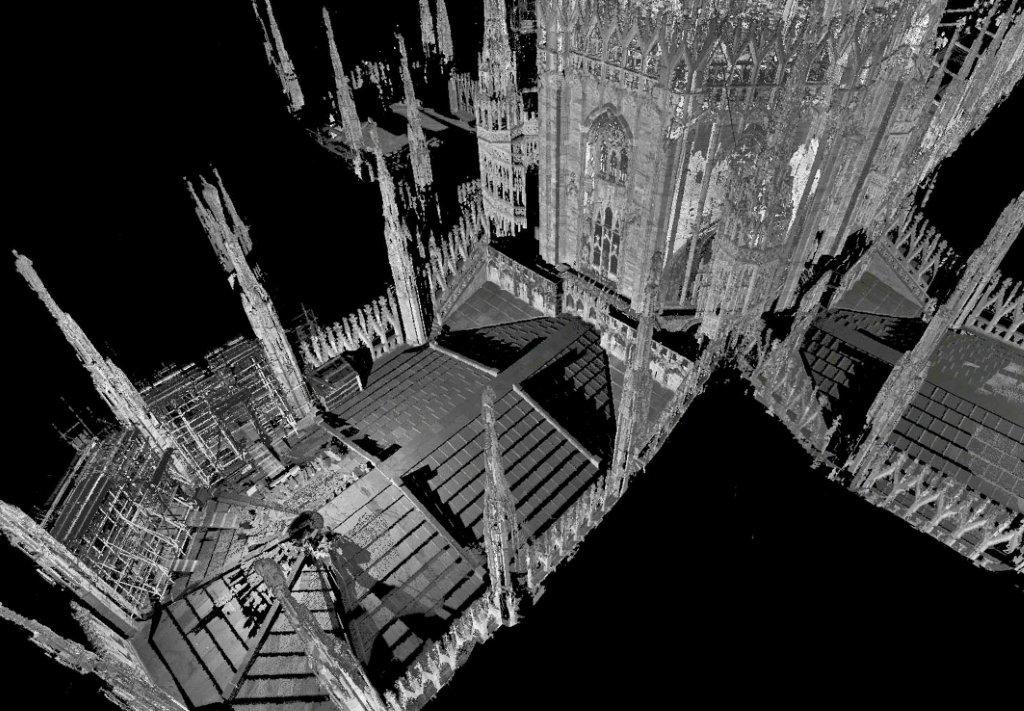
Volumetric data can be created through the use of thousands of images taken from slightly different perspectives. Microsoft's PhotoSynth was one of the first image processing systems capable of using millions of images in its models.
Because it is able to penetrate the tree canopy, imaging methods like LIDAR can be used to create detailed maps of the jungle. The cultural treasures found by archeologists mapping parts of Guatemala was more than anyone expected.
Medical Imaging Crash Course
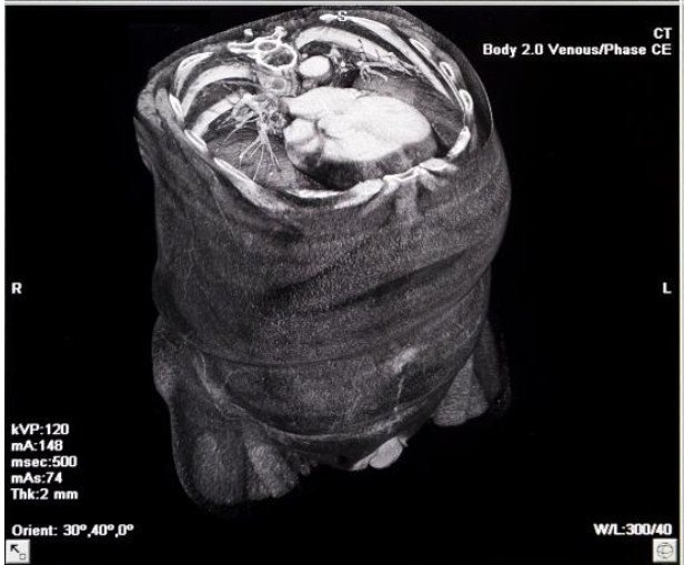
For this example, we will be using a set of CT images. Computed Tomography is a special type of x-ray imaging in which a narrow beam of radiation is quickly rotated around the body, producing a signal that is processed by a computer to create a a series of cross-sectional images (or slices) of the body. Because of how it is acquired and the ability to stack the slices, a CT scan has more information than a traditional (two-dimensional) x-ray.
When working with CT scans, you typically acquire and stack the images starting at a patient's feet and moving toward the head. CT scans have only a single channel of data, which makes them similar to grayscale images. Because the image is based on x-ray diffraction, the color (or intensity) of the image will be based on how dense the part of the body through which the x-ray passed was. Less dense tissue -- such as lung (which is mostly air), fat, or water -- will appear dark. More dense tissue -- such as muscle and bone -- will appear light.
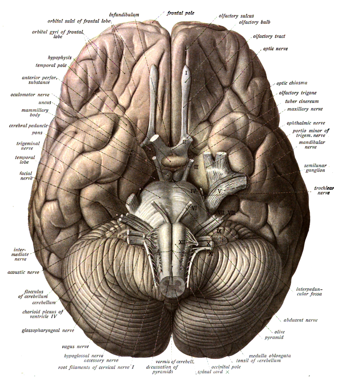
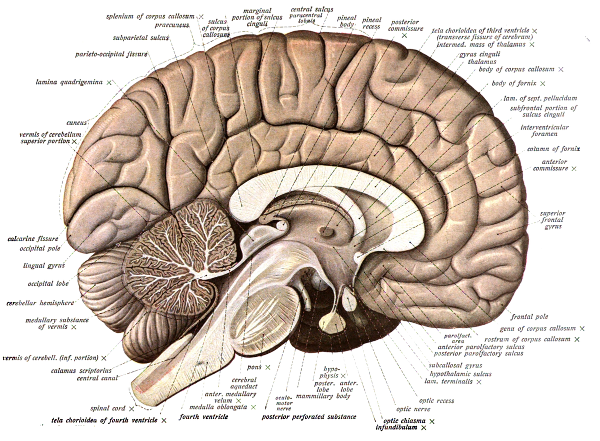
Anatomy Primer for Medical Imaging
To help us navigate the medical images we will be working with, it can be helpful to be familiar with the terminology of "views," since they relate to how images are acquired and navigated. Medical images are often described in terms of an "anatomical plane." While acquired in one plane, it is standard practice to re-sample and segment the views to other anatomical planes to allow doctors and researchers to look at the information from multiple perspectives.
The three most important anatomic planes are:
- Sagittal or median plane (also called the longitudinal or anteroposterior), which divides the body into left and right parts.
- Coronal or frontal plane (vertical) divides the body into dorsal and ventral (back and front, or posterior and anterior)
- Transverse or axial plane (lateral, horizontal) divides the body into cranial and caudal (head and feet)
CT images are only acquired in the axial plane. The dataset we will use in this article is of the upper abdomen and lower chest.
Working With Images Volumes in NumyPy
Like we've done previously, we will use NumPy to work with our imaging data and create the volume. This will require:
- Setting up dependencies needed for working with medical images and configuring the visualization tools we use in our analysis.
- Fetching a compressed archive of images from a remote source, extracting the data from an archive, and loading it to a NumPy array.
- Sample individual slices from the image for visualization in Python to determine what types of transforms should be performed.
- Create a panel figure to inspect the image series as a whole to ensure data consistency.
- Utilize simple techniques, such as a threshold to improve tissue contrast in the image.
- Creating a second panel figure to inspect the results.
Medical Imaging Data Formats
In comparison to the standard types of image formats -- JPEG, PNG, GIF -- that you may be familiar with, medical images use a special format called "Digital Imaging and Communications in Medicine" or DICOM. Since many traditional image processing libraries lack support for DICOM, we need to use a special library to read and parse the data.
There are many Python libraries that can load DICOM. Some of the most popular include pydicom and the Insight Toolkit (ITK). In this article, we will continue to use the imageio library which seen previously.
Import Dependencies
The codeblock below imports NumPy, SciKit-Learn, Seaborn, and other libraries. Some of the lmodules -- such as requests, io.BytesIO, seaborn, imageio, and matplotlib -- we have seen previously. Others are new:
skimageprovides a set of image processing tools built on top ofsklearnskimage.exposureincludes image processing algorithms which can help with modify the brightness and contrast (the exposure) of an image.skimage.morphologyincludes tool which can help to find the shape or morphology of features in an image. This includes such tasks as detecting boundaries or skeletons of objects.
# NumPy and plotting tools
import numpy as np
import matplotlib as plt
import seaborn as sns

# Utilities for working with remote data
import requests
from io import BytesIO
import zipfile

# Image processing shortcuts
import imageio

# SciKit-Image tools for working with the image data
from skimage import exposure
import skimage.morphology as morp
from skimage.filters import rank
Retrieve Data and Unpack to NumPy Array
Because medical imaging series can contain hundreds or thousands of files, it is common to create a single "archive" with all of the files and metadata about them kept together. The data we will be using has been packaged a zip archive.
The code in the listing below uses the zipfile module to allow us to work with the individual files inside of the archive and unpack them to NumPy. Specifically, we:
- Use
requeststo fetch the zip archive from the website where it is store. - Unpack the content of the request to a BytesIO file-like object and initialize a
ZipFileinstance so that it can be read and its contents accessed. - Once the data has been unpacked from the
ZipFile, we useimageioto load raw pixel data to a NumPy array as part of a comprehension.- Within the comprehension we iterate over the names of the files, which we retrieve using
namelist - We then retrieve a file-like object using the
openmethod of the zip file archivect_fdatathat can be read byimageio.imread.
- Within the comprehension we iterate over the names of the files, which we retrieve using
# Retrieve zip archive from website, create stream
ctr = requests.get(
    'https://oak-tree.tech/documents/156/example.lung-ct.volume-3d.zip')
ctzip = BytesIO(ctr.content)

# Create a  data in preparation of processing
ct_fdata = zipfile.ZipFile(ctzip)

# Load archived folder of DICOM image data
# The comprehension iterates through images and loads them to a stacked
# NumPy array. The
ct_idata = np.array(
    [imageio.imread(ct_fdata.open(fname)) for fname in ct_fdata.namelist()])
Once the data has been retrieved, we can check the shape of the NumPy array to ensure that it matches our expectation. There should be 99 layers of slices that are 512 pixels by 512 pixels.
Visualize CT Scan
Once the image data has been loaded, a good next step is to inspect the data and make decisions about what processing (if any) should be done.
Single Image
The code listing below pulls a single slice from the middle of the stack and renders it as a matplotlib figure.
# Show one sample image from the archive
plt.pyplot.figure(figsize=(8, 8), dpi=100)
plt.pyplot.imshow(ct_idata[15,:,:], cmap=plt.cm.gray)

# The coloring of the image is controlled by the plt.cm.gray.
# While color levels can be useful to visualize specific parts
# of an image, using gray helps with inspection in this type
# of a processing workflow.
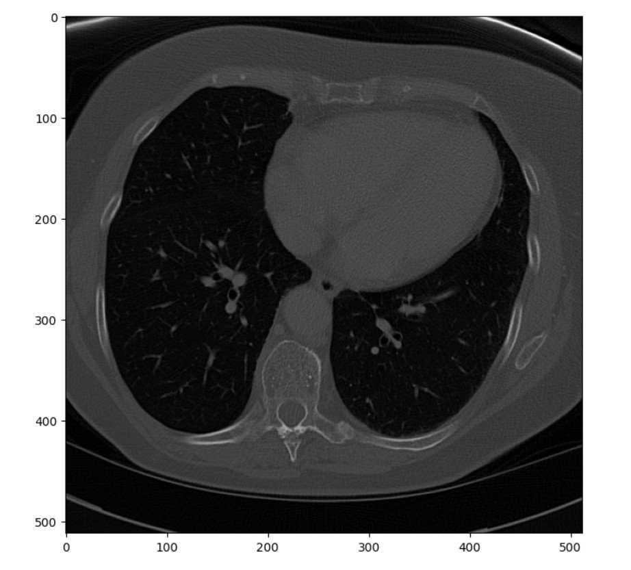
Image Series
The single image represents a pretty standard, unprocessed scan. It was selected more or less at random from the stack and happens to come from about mid-level in the chest. While completely adequate, it could be enhanced before being passed to a radiologist for reading or to a machine learning algorithm for segmentation. One common enhancement is to improve the contrast between different tissue types, such as bone and muscle. While some distinction between the tissues is visible in this image, it is subtle.
Before performing such processing, however, it is important to make sure that the images in the series are uniform. While CT is a pretty consistent imaging modality, it is not uncommon to get differences in pixel intensity between the layers. The quickest way to make such determinations is to sample the images in the scan and generate a panel plot with many images side-by-side.
The code in the listing below creates a helper method to manage visualization of the series. It takes a NumPy array with the data series and outputs a panel plot with a specified number of rows and columns.
- Because we only want to visualize part of the series, the method includes a parameter to control the size of the step:
sstep. It also provides a second parameter to control the number of columns the panel image should have:fcols. - From the panel and the size of the image series, the number of rows is calculated as
frows. If you haven't seen it before,//is the operator for integer division in Python 3. - The individual panels in the diagram are created using the
matplotlib.pyplot.subplotmethod. Each iteration through the sequence moves the figure to the next panel in the sequence. - The image is displayed using
imshow, again utilizing the grayscale color map.
# Helper method to generate panel series of CT image data

def display_series(idata, sstep=5, fcols=3, cmap=plt.cm.gray):
    ''' Create a sample panel to inspect the provided series as a whole.
        Samples images from the sequence based on the provided step.
        @input sstep (int, default=5): Number of images to skip when creating the
            series panel graphic.
        @input fcols (int, default=3): Number of columns to display in the
            panel graphic.
    '''
    frows = idata.shape[0]//sstep//fcols + 1

    for i,idx in enumerate(range(0, idata.shape[0], sstep)):
        sub = plt.pyplot.subplot(frows, fcols, i+1)
        sub.imshow(idata[idx,:,:], cmap=cmap)
Next we use the method to visualize the raw data.
# Create a sample panel to inspect the series as a whole
plt.pyplot.figure(figsize=(15,35))
display_series(ct_idata)
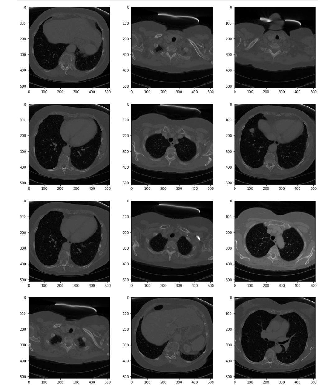
The series as a whole has "poor contrast." Pixel values are dark and the relative difference between types of tissue is small. The general pixel distribution between the slices, however, is consistent. This is a good candidate to enhance by increasing the contrast.
SciKit-Image includes a number of routines that can be used to optimize the image. Before applying any of them, looking at the pixel intensity histogram would be helpful in understanding the distribution of values before making choices.
The histogram can be quickly generated by flattening the whole volume and creating a Seaborn distplot. When working with a sequence of images, calculations and adjustments should be made on the volume as a whole.
# Plot histogram intensity for the entire volume. Working on the entire
# volume is desirable because it will allow for a uniform transform.
ct_idata_flat = ct_idata.flatten()
ct_px_min = ct_idata_flat.min()
ct_px_max = ct_idata_flat.max()

sns.distplot(ct_idata_flat)
plt.pyplot.title('Pixel Intensities', loc='left', fontsize=18)
plt.pyplot.title('Min: %s, Max: %s' % (ct_px_min, ct_px_max),
          loc='right', fontsize=13, color='grey')
Improving Contrast
Within CT images, the pixel values will often range from -1024 HU to 3000 HU. -1000 is no (or very minimal) defraction, associated with air. +3000 is associated with very high density objects, metal or contrast agent. Body tissues are somewhere in-between.
The histogram shows that there is a huge set of pixels corresponding to air and a second set corresponding to tissue. Removing the air and high contrast pixels would allow for the tissue contrast to increase. As a rule of thumb, gray-scale images look better when the left-hand edge of the useful pixel values are mapped to black and the right-hand edge of useful pixels is mapped to white. Re-mapping to this range is called "windowing" or "leveling." When done programmatically, it is sometimes called "contrast stretching."
In this part of the article, we will contrast stretch by doing a couple of things. First, we are going to throw away data we don't care about: very bright pixels and shades of gray currently encoded by air. Then, we will re-map the values so that there is more spread between the different tissue types.
Using a Threshold
We can throw away the useless data by creating a threshold with two cutoff points. While there are a lot of ways this might be implemented, here we will generate a boolean mask from the NumPy array selecting for values between two bounds: a lower bound and an upper bound.
From visual inspection of the histogram, air values seem to be less than -250. High contrast pixels appear to be above 1000 in intensity (or 1250, just to prevent the inadvertent exclusion of meaningful data).
As part of our processing, after we generate the mask, we will then shift all values by 1024 (the minimum value in the distribution) so that air (black) starts at 0. If the values are not shifted, when the boolean mask is applied all values will become 0. At present, "0" is in the middle of the tissue values.
# Apply contrast stretching to the image
ct_px_cutoff_lower = -250
ct_px_cutoff_upper = 1250

# Create threshold mask by applying lower/upper cutoffs
ct_bpfilter = (ct_idata > ct_px_cutoff_lower) & (ct_idata < ct_px_cutoff_upper)
With mask in hand, we can then do the shifting, apply the mask to values outside of our desired range (which sets their values to 0), and feed the resulting array into exposure.rescale_intensity which will increase the contrast between the new values.
# Shift range of all values based on the minimum.
# This sets the "air" reference to 0.
ct_idata1 = exposure.rescale_intensity(
    (ct_idata+abs(ct_px_min)) * ct_bpfilter,
    in_range=(550, ct_px_cutoff_upper+abs(ct_px_min)))
To see the results of the transformation, we can visualize the series using the same helper from earlier.
# Visualize the resulting transformation
plt.pyplot.figure(figsize=(15,35))
display_series(ct_idata1)
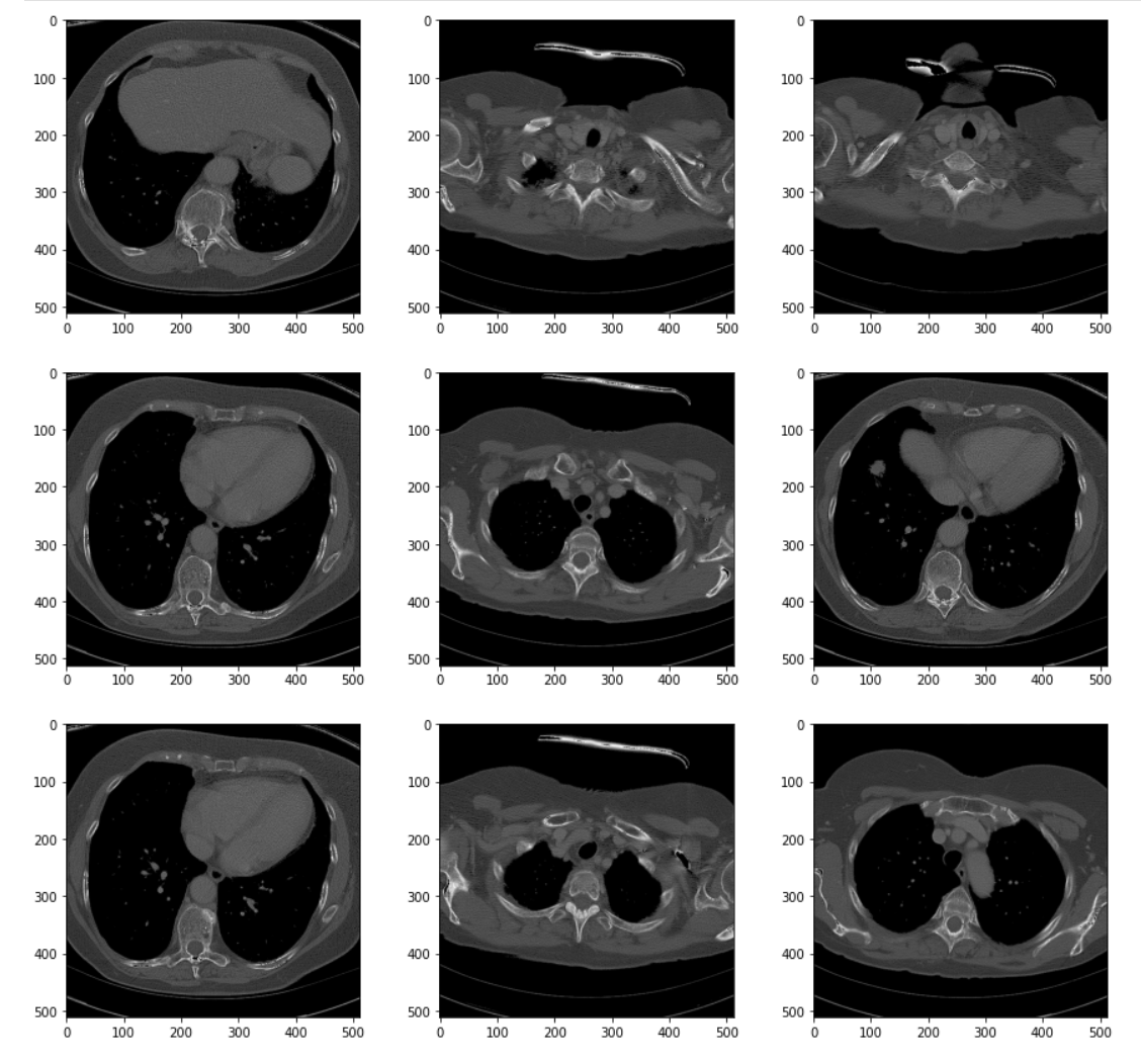
The processed images show better differentiation between the tissue types. It's easier to distinguish one type of soft tissue -- skin, fat, and muscle (for example) -- from others. The effects of the transforms become more obvious if we visualize the histogram of the transformed volume.
# Visualize the new histogram
plt.pyplot.figure(figsize=(8, 8))
sns.distplot(ct_idata1.flatten())
While this is a good start, even with the processing we've done the difference between tissues is still subtle. We could further stretch the contrast and apply other types of filters and max to further suppress artifact and noise. Nevertheless, we've taken a good first step.
Comments
Loading
No results found