Modeling Data with NumPy: Recognizing Hand-written Digits
For many types of machine learning problems, the way you structure (or model) data is important.
- For tabulated/structured data, choices in which features you include, how you combine them, and whether you normalize the the data will have a large impact on how the model behaves.
- When working work multi-media (such as image or audio) or signals data (such as EKG), decisions such as how to sample, whether to normalize, and how to combine signals from various channels have huge implications in how you build your models and the systems around it.
- For Natural Language Processing (NLP) systems, how you approach tokenization, parsing, and representation generally determine the success and failure of your model.
Put succinctly, trying to gain insight from data requires you to make (sometimes hard) decisions how to structure and model it. In this article, we will look at how transforming images which show handwritten digits enables us to create a classical machine learning model capable of classifying them with very high accuracy.
This example has been adapted from one included in the SciKit-Learn manual. It is Part 3 of a larger series showing how NumPy can be used to model data for machine learning. If you have not already done so, checkout Part 1, which provides an overview of NumPy and how to work with image data. A Jupyter notebook with the code in the article can be downloaded here. A Docker environment with NumPy, Pandas, and other dependencies needed to run the code can be found here.
Recognizing Handwritten Digits
The United States Postal System processes nearly two-hundred million pieces of First-class mail each day. To ensure that letters are sorted and delivered accurately, it uses computer vision systems to read the addresses to which a letter should be sent and route it correctly.
When building a classifier to identify digits or other letters, you need to:
- Scan the handwritten digits using a camera or another form of optical input.
- "Segment" the compound image into a new image with one letter in each.
- Utilize image processing algorithms or build a multi-class classifier on the raw grayscale pixels capable of predicting which digit is present.
MNIST
MNIST is one image dataset that has been used in the creation of such computer visions systems. It is composed of handwritten digits with a training set of 60,000 examples and a test set of 10,000 more. It is considered the "Hello World" of computer vision, and is often used as a benchmark of multi-class classification systems. It is such a prominent dataset, in fact, that it is included in the datasets module of SciKit-Learn.
While there are many approaches that can be used to extract features from the data, a surprisingly accurate model can be built by using the integer pixel intensity values. For our data model, we will flatten the images to a vector with sixty four input features, one for each of the pixels in the 8x8 pixel images. For the "target", we will use the digit contained in the image, giving us known labels ranging in value from 0 to 9.
Machine Learning Workflow
The example code in this article is fairly representative of many machine learning workflows. In building most any ML model, it is necessary to:
- Load data from a source and verify the structure.
- Make decisions about how the data should be represented in the model. For structured data, this usually means converting features to numeric values and representing all data points as a vector of defined size. For image data, it means flattening the image and combining with other desired components.
- Split the data into a testing and training set. The training set is used to build the model while the testing set is used to assess it. It is a very bad idea to assess a model using the same data used to train it.
- (optional) Train alternative models to understand how different algorithms perform against one another.
- Tune the algorithm's initialization parameters (sometimes called hyperparameters) to tweak the model's accuracy.
In the code throughout this article we will follow this general recipe. We will load the MNIST data from sklearn, visualize samples using matplotlib, split the data into a testing and training set, train a pair of machine learning models, and assess the accuracy.
Import Dependencies and Configure Visualization
The codeblock below imports NumPy and the helper utilities used in the example. This includes methods from a number of SciKit-Learn modules:
sklearn.datasetsprovides helpers to retrieve the data and load it as NumPy n-dimensional arrays.sklearn.svmprovides the implementation of Support Vector Machines, which will be used as one of the ML classifiers. The Support Vector ClassifierSVCclass will be used.sklearn.ensembleprovides theRandomForestClassifierwhich will be used as an alternative ML classifier for comparison.- for creating the train/test split,
train_test_splitfrom thesklearn.model_selectionmodule will be used.model_selectionadditionally contains tools for helping to validate and optimize models, though their use will be omitted here.
import numpy as np
import matplotlib.pyplot as plt

# sklearn includes a complement of datasets which can be used
# to explore different types of machine learning examples
from sklearn import datasets

# SVM: Support vector machine
from sklearn import svm

# Ensemble/RandomForestClassifier
from sklearn.ensemble import RandomForestClassifier

# sklearn.metrics helps to quantify the quality of predictions
# See https://scikit-learn.org/stable/modules/model_evaluation.html
from sklearn import metrics
from sklearn.model_selection import train_test_split
Load Data from SciKit-Learn
The code listing below retrieves the images and loads them as a set of 8x8 pixel images layered on top of one another in a NumPy multidimensional array. The sample included with sklearn.datasets has 1797 samples.
# MNIST is a set of hand-drawn numbers encoded in 8x8 pixel images.
# It is considered the "Hello World" of computer vision, and for that
# reason it is included in the set of data distributed with SciKit-Learn.
digits = datasets.load_digits()
Visualize Images from the Dataset
After loading the data, it's always a good idea to inspect the information to ensure that it matches expectations. The code listing below:
- combines the images and data into a combined structure for visualization
zipis useful for combining elements from multiple iterables into a single object. It works by iterating over the containers and pulling elements from the same index into a tuple which gets returned iteratively. It will stop iteration when it reaches the end of the shortest container.
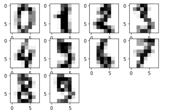
- creates a panel plot showing a sample of ten images
plt.subplotis used to create a 3x4 panel plot iteratively. The active panel is controlled by a counter provided byenumerate.- The subplot instance
subis then used to plot the image dataidata.
# Pull the first nine images from the images and their associated targets
example_images = tuple(zip(digits.images[:10], digits.target))

# Create a figure showing the images
for i, (idata, ilabel) in enumerate(example_images):
    sub = plt.subplot(3, 4, i+1)
    sub.imshow(idata, cmap='Greys')
Create Classification Model to Predict Digits
As noted above, to train a classifier for the image data, we need to flatten the two-dimensional arrays to a single dimension. After the data has been flattened and re-shaped to a two-dimensional array with one sixty-four element vector for each image, we are ready to initialize and train a classifier.
Re-shape Data for ML Input
In the code listing below, we utilize the reshape method to transform the input array.
- The structure of the resulting data will be the number of samples (determined by taking the length of the input structure) and the squashing of the interior structure.
- Using
-1for the second transform tells NumPy to infer the length of the row dimension from the remaining dimensions in the structure. See the SciPy documentation for details.
# Flatten the structure of the array using reshape
# -1 tells NumPy to determine the row size from the
# length of the inner dimensions.
mnist_mldata = digits.images.reshape((len(digits.images), -1))
Create Machine Learning Model: Support Vector Classifier SVC
To generate the machine learning model, we will follow the general recipe described above:
- Split data into training/testing sets
- Initialize the machine learning algorithm
- Train model instance on data:
fit - Assess model performance:
score
Support Vector Machines use a linear model for classification problems and a "kernel" to help it fit the data to the outcome classes. For classification, the SVM attempts to create a "line" (or hyperplane for higher-order datasets) which separate the data into specific classes matching the training labels. See Support Vector Machines: An Overview for details.
# Step 1: Split data into training/testing sets
X_train, X_test, y_train, y_test = train_test_split(
    mnist_mldata, digits.target, test_size=0.3, shuffle=False)
Note: When creating the testing/training splits that we did not shuffle the data. This was done to preserve ordering so that the original data can be retrieved for visualization.
# Step 2: Initialize machine learning algorithm
mnist_svm = svm.SVC()

# Step 3: Train model instance on the data
mnist_svm.fit(X_train, y_train)

# Step 4: Assess model performance on the testing data
mnist_svm.score(X_test, y_test)
The SVC learning model does a very good job of fitting the data to the target. It is able to accurately identify more than 95% of the testing data correctly!
Alternative Classification Algorithm: Random Forest
When working with a classification problem, it is often useful to compare multiple algoritms against one another to see relative performance.
# Initialize model instance, fit training data, assess
mnist_rf = RandomForestClassifier()
mnist_rf.fit(X_train, y_train)
mnist_rf.score(X_test, y_test)
While also very accurate, the RandomForestClassifier is slightly less accurate than the SVC instance.
Apply Model to Data and Visualize Results
To get a sense of how the algorithm performed, let's visualize samples of the model's performance. The example code below uses the SVC model to create a set of predictions and plot the images with the predicted and actual labels. When we created the testing and training datasets, we didn't shuffle the data. This allows us to pull the images from the original array for visualization.
# Apply SVC model to create a set of "predictions"
predictions_svm = mnist_svm.predict(X_test)

# Create a structure including sample images, predictions, and labels
example_predictions_svm = tuple(
    zip(digits.images[len(X_train):], predictions_svm, y_test))

# Check resulting structure to ensure that data combined correctly
example_incorrect_predictions_svm = tuple(
    filter(lambda v: v[1] != v[2], example_predictions_svm))
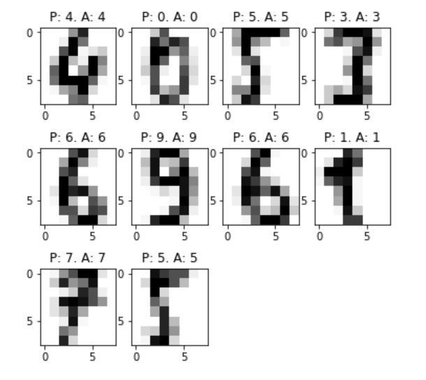
Correctly Matched Images
plt.figure(figsize=(6, 6))

# Visualize correctly matched images
for i, (idata, p, ilabel) in enumerate(example_predictions_svm[:10]):
    sub = plt.subplot(3, 4, i+1)
    sub.imshow(idata, cmap='Greys')
    plt.title('P: %s. A: %s' % (p, ilabel))
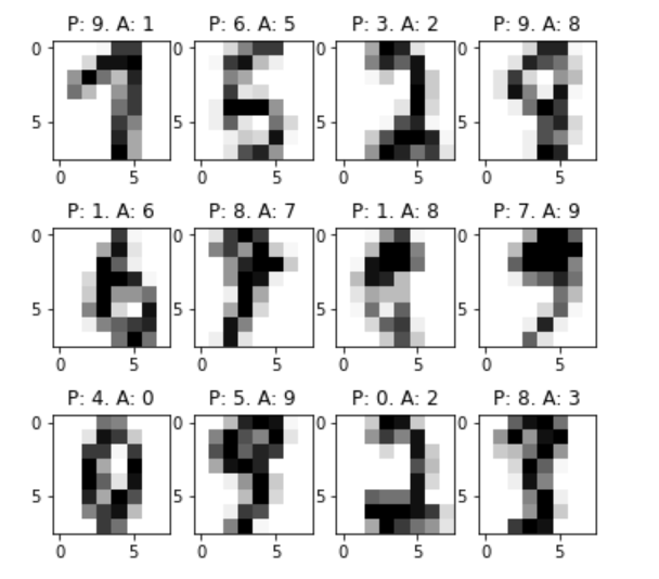
Incorrectly Matched Images
plt.figure(figsize=(6, 6))

# Visualize correctly matched images
for i, (idata, p, ilabel) in enumerate(example_incorrect_predictions_svm[:12]):
    sub = plt.subplot(3, 4, i+1)
    sub.imshow(idata, cmap='Greys')
    plt.title('P: %s. A: %s' % (p, ilabel))
Comments
Loading
No results found